Usage¶

This page shows how to work with GraphCoreSGHDBSCAN in practice after the package is installed.

The package supports two main workflows:

build a similarity graph from feature data and cluster from that graph
provide a graph or adjacency representation directly in precomputed mode

For most users, GraphCoreSGHDBSCAN is the main entry point.

Basic workflow¶

A typical workflow is:

prepare a feature matrix X or a precomputed graph
create a GraphCoreSGHDBSCAN model
call fit(...) or fit_predict(...)
inspect labels
inspect the condensed tree
compare several min_samples values if needed

Minimal example¶

The simplest usage pattern is:

from coresg_graphhdbscan import GraphCoreSGHDBSCAN

model = GraphCoreSGHDBSCAN()
labels = model.fit_predict(X)

This uses the default configuration:

min_samples=10
sim_graph_method="sc_umap"
metric="euclidean"
metric_kwds=None
add_neighbor=True
no_noise=True
n_neighbors=15
heuristic_connect=False
min_cluster_size=None

fit vs. fit_predict¶

Use fit_predict(X) when you want labels immediately for a single requested configuration.

model = GraphCoreSGHDBSCAN(min_samples=10)
labels = model.fit_predict(X)

Use fit(X) when you want to inspect the fitted object, view the hierarchy, or retrieve results for several min_samples values later.

model = GraphCoreSGHDBSCAN(min_samples=10)
model.fit(X)

Single `min_samples` value¶

If you want one clustering solution only, pass a single integer:

model = GraphCoreSGHDBSCAN(min_samples=10)
labels = model.fit_predict(X)

This is the simplest and most common starting point.

Multiple `min_samples` values in one run¶

One of the package’s main strengths is the ability to fit several min_samples values in one model run.

from coresg_graphhdbscan import GraphCoreSGHDBSCAN

model = GraphCoreSGHDBSCAN(min_samples=[5, 10, 15])
model.fit(X)

labels_5 = model.labels_for(5)
labels_10 = model.labels_for(10)
labels_15 = model.labels_for(15)

This is useful when you want to compare clustering behavior across several density settings without rebuilding the full workflow from scratch.

You can also use ranges:

model = GraphCoreSGHDBSCAN(min_samples=range(2, 10))
model.fit(X)

Inspecting the hierarchy¶

After fitting, you can inspect the hierarchical structure through the condensed tree.

Static condensed tree¶

The most reliable visualization method is the static condensed tree:

model.fit(X)
model.plot_condensed_tree(10)

If you fit several min_samples values, pass the specific value you want to inspect.

Interactive condensed tree¶

For live notebook work, the package also provides an interactive condensed tree:

widget = model.interactive_condensed_tree()
widget

This view lets you change min_samples interactively and inspect the corresponding condensed tree without refitting the model. It is useful when you fit several min_samples values in one run and want to compare the resulting hierarchies visually.

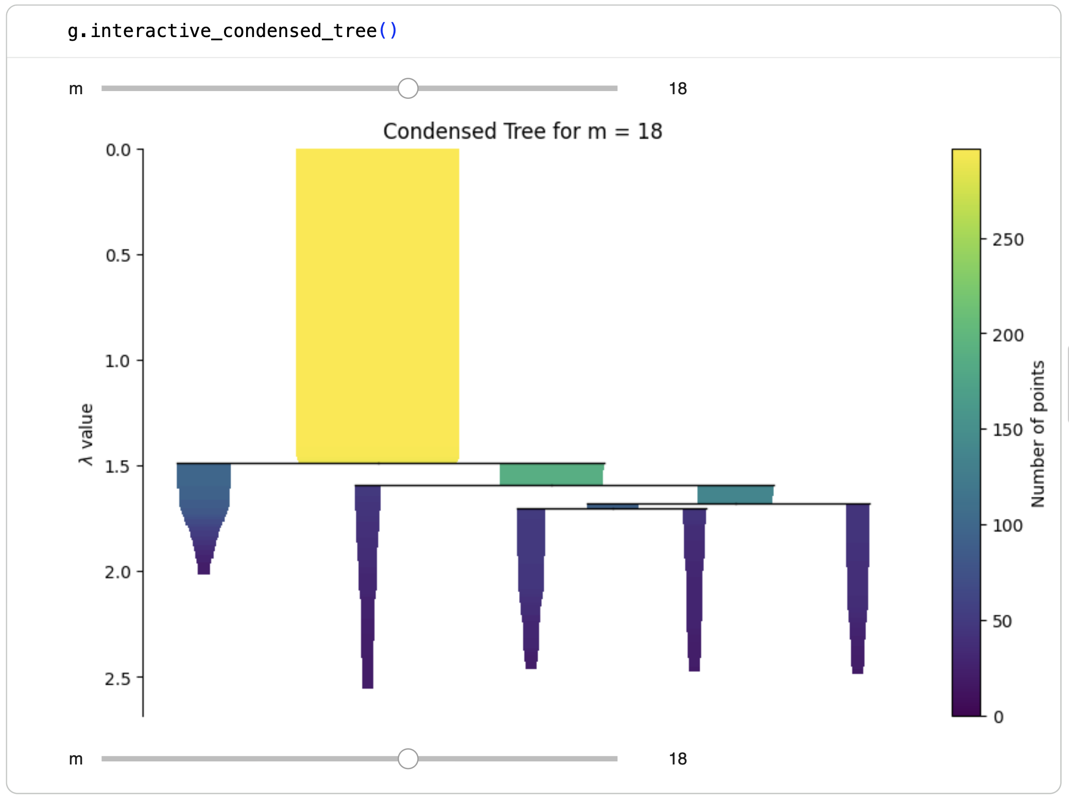
Interactive condensed tree widget with a slider for min_samples and a condensed tree display.

In this interface, the slider controls the selected value of min_samples. As the selected value changes, the displayed condensed tree updates so that you can compare hierarchical structure across different density settings.

A typical workflow is:

model = GraphCoreSGHDBSCAN(min_samples=range(2, 20))
model.fit(X)

widget = model.interactive_condensed_tree()
widget

This feature is most useful in a live Jupyter environment.

Choosing a graph-construction backend¶

The package supports several graph-construction backends through sim_graph_method.

Default UMAP-style graph¶

model = GraphCoreSGHDBSCAN(
    sim_graph_method="sc_umap",
    n_neighbors=15,
)
model.fit(X)

This is the default and a good starting point for many datasets.

Gaussian connectivity graph¶

model = GraphCoreSGHDBSCAN(
    sim_graph_method="sc_gauss",
    n_neighbors=15,
)
model.fit(X)

This uses Scanpy’s Gaussian connectivity routine.

PhenoGraph-style graph¶

model = GraphCoreSGHDBSCAN(
    sim_graph_method="jaccard_phenograph",
    n_neighbors=15,
)
model.fit(X)

This uses a PhenoGraph-style graph construction.

Using different distance metrics¶

The metric parameter controls the distance measure used during similarity graph construction.

The default is:

model = GraphCoreSGHDBSCAN(
    sim_graph_method="sc_umap",
    metric="euclidean",
)

model.fit(X)

Other supported distance metrics include:

"cityblock"
"cosine"
"euclidean"
"l1"
"l2"
"manhattan"
"braycurtis"
"canberra"
"chebyshev"
"correlation"
"dice"
"hamming"
"jaccard"
"mahalanobis"
"minkowski"
"rogerstanimoto"
"russellrao"
"seuclidean"
"sokalmichener"
"sokalsneath"
"sqeuclidean"
"yule"
"hybrid_euclidean_cosine"

Cosine distance¶

model = GraphCoreSGHDBSCAN(
    sim_graph_method="sc_gauss",
    metric="cosine",
)

model.fit(X)

Correlation distance¶

model = GraphCoreSGHDBSCAN(
    sim_graph_method="sc_umap",
    metric="correlation",
)

model.fit(X)

Minkowski distance with metric_kwds¶

Some metrics require additional keyword arguments. These can be passed through metric_kwds.

model = GraphCoreSGHDBSCAN(
    sim_graph_method="sc_umap",
    metric="minkowski",
    metric_kwds={"p": 1.5},
)

model.fit(X)

Mahalanobis distance¶

For Mahalanobis distance, pass the inverse covariance matrix VI:

import numpy as np

VI = np.linalg.pinv(np.cov(X, rowvar=False))

model = GraphCoreSGHDBSCAN(
    sim_graph_method="sc_umap",
    metric="mahalanobis",
    metric_kwds={"VI": VI},
)

model.fit(X)

Standardized Euclidean distance¶

For standardized Euclidean distance, pass the variance vector V:

import numpy as np

V = np.var(X, axis=0, ddof=1)

model = GraphCoreSGHDBSCAN(
    sim_graph_method="sc_umap",
    metric="seuclidean",
    metric_kwds={"V": V},
)

model.fit(X)

Hybrid Euclidean-cosine mode¶

model = GraphCoreSGHDBSCAN(
    sim_graph_method="sc_umap",
    metric="hybrid_euclidean_cosine",
)

model.fit(X)

In this mode, full distances remain Euclidean while neighborhood graph construction uses cosine geometry.

Unsupported metric and combination¶

The metric "kulsinski" is not supported because it is not available in current versions of scikit-learn’s pairwise_distances.

The following combination is intentionally not supported:

GraphCoreSGHDBSCAN(
    sim_graph_method="sc_gauss",
    metric="yule",
)

This combination can produce non-finite graph weights. Use metric="yule" with sim_graph_method="sc_umap" or sim_graph_method="jaccard_phenograph" instead.

Using precomputed graphs¶

If you already have a graph or adjacency representation, use sim_graph_method="precomputed".

model = GraphCoreSGHDBSCAN(
    min_samples=10,
    sim_graph_method="precomputed",
    no_noise=True,
)
model.fit(my_graph)

In precomputed mode, the input to fit(...) may be:

a networkx.Graph
a SciPy sparse adjacency matrix
a square dense adjacency matrix

This mode is useful when the graph is already part of the experimental design or has been built by another method.

Connectivity handling¶

The final graph used by clustering must be connected.

Default behavior¶

With heuristic_connect=False, disconnected components are connected using a simple fallback that adds synthetic bridge edges.

model = GraphCoreSGHDBSCAN(
    heuristic_connect=False,
)

Heuristic connectivity¶

With heuristic_connect=True, the package increases n_neighbors until the graph becomes connected.

model = GraphCoreSGHDBSCAN(
    heuristic_connect=True,
    n_neighbors=15,
)

During fitting, the package may report messages such as:

Trying n_neighbors = 16
Trying n_neighbors = 17

Noise reassignment¶

With no_noise=True, points initially labeled -1 are reassigned by an MST-based propagation step after clustering.

model = GraphCoreSGHDBSCAN(
    no_noise=True,
)

If you want to preserve the original HDBSCAN*-style noise labels, disable it:

model = GraphCoreSGHDBSCAN(
    no_noise=False,
)

Useful outputs after fitting¶

After fitting, users commonly inspect:

model.coresg_ for the internal CoreSG object
model.similarity_graph_ for the initial similarity graph
model.similarity_graph_WSS for the weighted structural similarity graph
model.dissimilarity_graph_ for the graph after similarity-to-dissimilarity conversion
model.connected_graph_ for the final connected graph
model.dist_matrix_ for the dense matrix used by CoreSGHDBSCAN

If you fit multiple min_samples values, retrieve a selected solution with:

labels = model.labels_for(10)

For lower-level access, labels are also stored inside the internal model objects associated with each fitted min_samples value.

Common usage patterns¶

Default configuration¶

from coresg_graphhdbscan import GraphCoreSGHDBSCAN

model = GraphCoreSGHDBSCAN()
labels = model.fit_predict(X)

Explore several density settings¶

model = GraphCoreSGHDBSCAN(
    min_samples=range(2, 20),
    sim_graph_method="sc_gauss",
    n_neighbors=16,
    no_noise=True,
    metric="euclidean",
    heuristic_connect=True,
)

model.fit(X)
model.plot_condensed_tree(4)
labels_18 = model.labels_for(18)

Cosine-based graph construction¶

model = GraphCoreSGHDBSCAN(
    min_samples=[5, 10],
    sim_graph_method="sc_gauss",
    metric="cosine",
    n_neighbors=20,
)
model.fit(X)
labels_10 = model.labels_for(10)

Precomputed graph workflow¶

model = GraphCoreSGHDBSCAN(
    min_samples=10,
    sim_graph_method="precomputed",
    no_noise=True,
)
model.fit(my_graph)
model.plot_condensed_tree(10)

Working with fitted results¶

After calling fit(), the package stores results for each fitted min_samples value.

g = GraphCoreSGHDBSCAN(
    min_samples=range(2, 20),
    sim_graph_method="sc_gauss",
    metric="euclidean",
    n_neighbors=16,
    no_noise=True,
    save_models=True,
)
g.fit(X)

Stored labels¶

labels_5 = g.labels_by_m_[5]

You can also use:

labels_5 = g.labels_for(5)

Note that labels_for(m) may apply noise reassignment depending on the no_noise setting, while labels_by_m_[m] is the directly stored fitted result.

Stored condensed trees¶

tree_5 = g.condensed_trees_[5]

Plot a selected condensed tree:

g.plot_condensed_tree(5)

Interactive condensed tree browser:

g.interactive_condensed_tree()

Stored models¶

If save_models=True, full per-m models are available:

model_5 = g.models_[5]

Practical notes¶

min_samples is the main clustering hyperparameter and is often the first thing to tune.
min_cluster_size=None means that the package follows the selected min_samples value for each run.
plot_condensed_tree(...) is the most reliable visualization for static documentation and reports.
interactive_condensed_tree() is best suited for live notebooks.
Some graph builders depend on optional packages and will raise an import error if those packages are not installed.

Notebook tip¶

In notebook environments, use a trailing semicolon to suppress the display of the fitted object representation:

g.fit(X);