Example: Hierarchical clustering on a CITE-seq dataset

This notebook presents a structured GraphHDBSCAN workflow on a CITE-seq dataset.

Sections:

1. installation

2. imports and setup

3. data loading / preparation

4. model construction and fitting

5. condensed tree visualization

6. optional interactive exploration

Installation

These commands are only required when running the notebook in a fresh environment.

Install required package(s):

!pip install git+https://github.com/Campello-Lab/GraphHDBSCAN.git

Build and fit the model

Configure GraphHDBSCAN, fit the model, and inspect the resulting hierarchical clustering state.

from coresg_graphhdbscan import GraphCoreSGHDBSCAN

/usr/local/lib/python3.12/dist-packages/hdbscan/robust_single_linkage_.py:175: SyntaxWarning: invalid escape sequence '\{'
  $max \{ core_k(a), core_k(b), 1/\alpha d(a,b) \}$.

Load and prepare the dataset

Load the CITE-seq data and prepare the representation used by the clustering pipeline.

import scanpy as sc
adata =  sc.read_h5ad("/content/T_cells_CiteSeq_GEX_processed.h5ad") #file path
count_matrix = adata.X #cells as rows and genes as columns
true_labels = adata.obs['cell_labels']

g = GraphCoreSGHDBSCAN(
    min_samples=range(2,6),
    sim_graph_method="sc_umap",
    n_neighbors=7,
    no_noise=True,
    metric="euclidean",
    min_cluster_size=55,
)

g.fit(adata.X)

[CORE-SG] (precomputed) CORE-SG graph has 20841 edges
[CORE-SG] m= 2: MST+tree+labels in 0.1340s
[CORE-SG] m= 3: MST+tree+labels in 0.1288s
[CORE-SG] m= 4: MST+tree+labels in 0.1228s
[CORE-SG] m= 5: MST+tree+labels in 0.1331s

GraphCoreSGHDBSCAN(min_samples_list=[2, 3, 4, 5], metric='euclidean', eps=1e-12, min_cluster_size=55, X_=None, N_=None, D_=None, core_={}, kmax_=None, edges_ut_=None, idx_with_self_=None, dst_with_self_=None, idx_no_self_=None, dst_no_self_=None, A_knn_=None, msts_={}, mst_times_={}, models_={}, times_={})

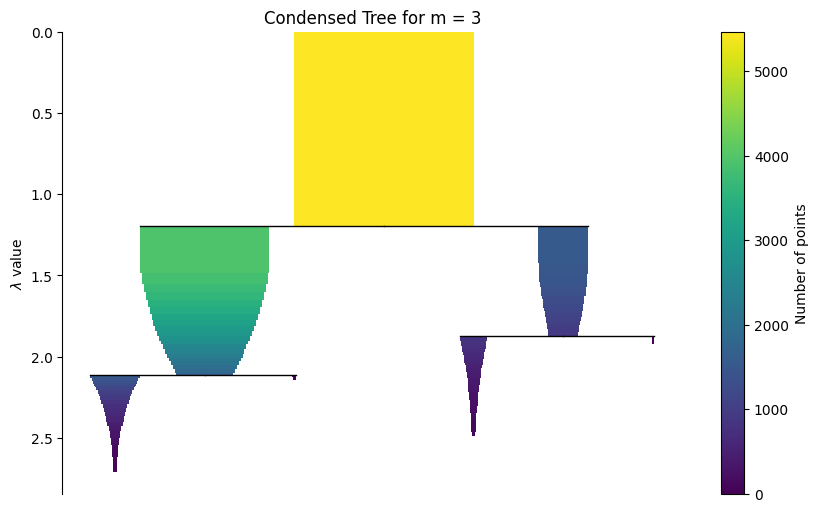
Visualize the hierarchy

A static condensed tree is included first for reliable rendering in the documentation. The interactive widget is shown afterwards for live notebook use.

g.plot_condensed_tree(3)

<Axes: title={'center': 'Condensed Tree for m = 3'}, ylabel='$\\lambda$ value'>

The widget below is most useful in a live Jupyter environment.

g.interactive_condensed_tree()